Coursework · Data Engineering and Analysis

Credit Scoring

Credit default classifier where a missed default costs ten times more than a wrong refusal. The threshold and the model are both optimized for that asymmetric cost. MLflow registry, Docker serving, SHAP explanations, pytest tests.

Context

The Data Engineering and Analysis module at ESAIP gives a multi-week project on a real-world ML deployment scenario. The subject was credit scoring on the Kaggle Home Credit Default Risk dataset: seven CSVs to merge, a 92/8 class imbalance, an asymmetric business cost imposed by the brief — a missed default ten times worse than a wrong refusal — and an end-to-end MLOps pipeline expected from data prep through Docker serving.

Team of three. I owned the data engineering layer end-to-end — multi-table merge, schema validation, feature engineering, stratified train/valid/test split, preprocessing — and the MLflow architecture wired into every training run (experiments, runs, model registry, artifacts, optimal threshold persisted alongside the model). My teammates handled the modeling and SHAP explainability.

The problem

Defaults are rare in this dataset — about 8% of clients — so accuracy is misleading from the start. The brief makes it harder: a missed default costs ten times more than a wrong refusal, so the model can't be evaluated on AUC alone, and the standard 0.5 decision threshold won't be optimal by default. And every refusal must be justifiable to the customer, so we can't ship a black box. Three constraints, three explicit responses in the pipeline.

The approach

The data engineering layer reads seven CSVs (application, bureau, bureau_balance, previous_application, POS_CASH, installments, credit_card), merges them with explicit duplicate checks and primary-key validation, normalizes types via a YAML schema, and creates business features (payment rate, annuity-to-income ratio, days-employed-percent). Stratified split 60/20/20 preserves the 92/8 class distribution everywhere. Winsorization at IQR×5 for outliers, median or mode imputation, and one-hot encoding for categoricals. Outputs go to Parquet so reload is fast and reproducible.

The modeling layer runs a Logistic Regression baseline and a LightGBM tuned with Optuna under stratified K-fold cross-validation. class_weight = balanced handles the imbalance natively. Every run logs to MLflow: parameters, AUC, recall on the minority class, business cost, the model itself, the optimal threshold, and the SHAP plots — so the registry can be queried by "minimum business cost" rather than "best AUC".

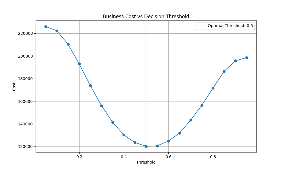
Optimizing the threshold

The default 0.5 threshold is not automatically right when the costs are asymmetric. The pipeline sweeps the threshold from 0.05 to 0.95 and computes the total business cost (10 × FN + 1 × FP) at each point, then persists the threshold that minimizes it. On this run the optimum landed at 0.5, but the cost rises sharply on either side — a small drift in calibration would have cost real money. The threshold and the model are stored together; moving the model without its threshold would silently break the calibration.

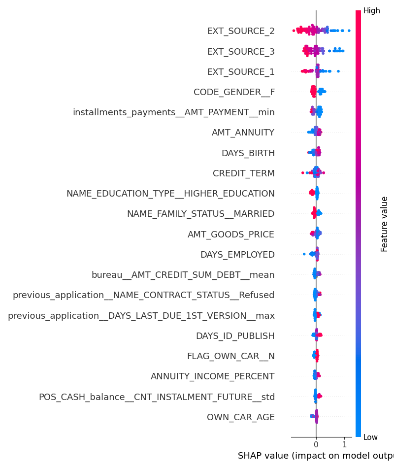
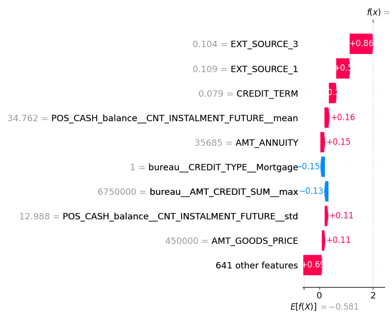
Line chart showing total business cost as a function of the decision threshold, with a clear minimum at threshold 0.5 and the cost rising sharply at lower and higher thresholds. — Business cost as a function of the decision threshold. The optimum landed at 0.5 here, but the curve is steep on both sides.

Explainability

A regulated refusal needs to be defensible per case, not in aggregate. SHAP TreeExplainer produces both a global feature ranking — the dataset-wide contribution of each feature — and a local waterfall plot for any individual decision. The top three features are external credit scores (EXT_SOURCE_2, EXT_SOURCE_3, EXT_SOURCE_1), followed by demographic and payment-history signals. For a specific refusal, the local plot shows exactly which feature values pushed the score up or down, and by how much.

SHAP summary plot ranking the most important features across the test set, with EXT_SOURCE_2, EXT_SOURCE_3 and EXT_SOURCE_1 at the top. — Global SHAP feature importance over the test set.

SHAP waterfall plot for a single refused application, showing each feature's contribution to the model output relative to the dataset baseline. — Local SHAP waterfall for a single refused application — the contribution of each feature value to that specific decision.

Result

Final AUC of 0.7862 on the held-out test set, with a business cost of 29,680. Validation AUC was 0.7781, so the test result generalized cleanly. The brief flagged overfitting risk above AUC 0.82 — landing at 0.79 means the model is honest, not chasing the leaderboard. The Optuna search across 20 trials converged on a decision threshold of 0.5, identical to the default; on this dataset the cost asymmetry happens to be calibrated by the model's natural probability output, but the search was the only way to confirm it rather than assume.

Around the model

The infrastructure around the model: an MLflow registry where every run carries the model, the optimal threshold, and the SHAP plots as versioned artifacts; a Docker image that serves the model behind POST /invocations on port 1234, using mlflow models serve with no extra framework; a pytest suite covering data prep invariants and MLflow utilities. Configuration lives in YAML files validated against a schema, so config drift fails loudly rather than silently. Each piece had a written spec before any code.