Coursework · Explainable AI

Explainable AI

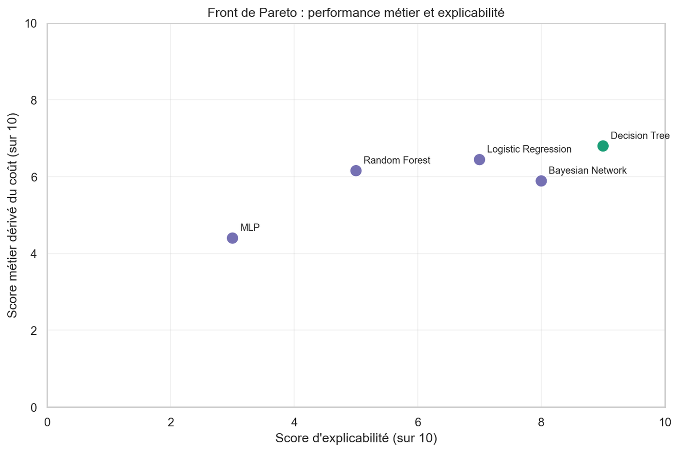
Pareto comparison of five models for credit approval — business cost vs explainability. The MLP wins on accuracy and loses everywhere else. The Decision Tree dominates the frontier: lowest cost, highest auditability, the only non-dominated point.

Context

The Explainable AI module at ESAIP gives one week to build and present a credit-approval recommendation. The deliverable is a sales pitch: convince a fictional client — a bank's risk director — that your model choice is the right one. The dataset is UCI German Credit, 1000 clients, 700 Good / 300 Bad. The team picked the cost asymmetry from the dataset's original cost matrix — a missed default costs five times more than a wrongly refused good client.

Team of three. I owned the MLP and the Pareto computation. My teammates handled the four other models — Decision Tree, Logistic Regression, Random Forest, Bayesian Network — and their explainability layers.

The problem

Five candidate models, five different explainability stories. A MLP is opaque but accurate. A Random Forest needs SHAP and a surrogate tree to be readable. A Logistic Regression has interpretable coefficients but assumes linearity. A Bayesian Network exposes a causal DAG and conditional probability tables, but the lecture is technical. A Decision Tree is auditable directly — the rules are the model. Picking one means trading accuracy against the kind of explanation a bank director can defend in front of a regulator.

The approach

All five models are evaluated at the same cost-sensitive threshold. The German Credit cost matrix says a false negative costs five, a false positive costs one. Standard 0.5 thresholding ignores this asymmetry. The cost-minimizing threshold is P(Bad) ≥ 1/6 ≈ 0.167 — refuse anyone whose default probability exceeds one in six. Same threshold across all five models keeps the comparison fair.

Each model gets a tailored explainability layer: SHAP for feature importance, a surrogate tree to approximate the Random Forest and the MLP into a readable form, an expert DAG plus a learned DAG (HillClimbSearch with BIC-d) plus conditional probability tables for the Bayesian Network. The Decision Tree and Logistic Regression are interpretable directly. The explainability score is a 1–10 grid evaluated by the team against a checklist: auditability, lisibility, stability of explanations, ability to defend each prediction to a non-technical stakeholder.

Result

At the cost-sensitive threshold, the Decision Tree had the lowest business cost (0.480, 5 risky clients accepted out of 90) and the highest explainability score (9/10). The MLP had the highest accuracy (0.693) but the highest cost (0.840) — it accepted 40 risky clients, the worst result of the five. The Random Forest was the safest in absolute terms (only 3 risky accepts) but refused 158 good clients, pushing its mean cost to 0.577. The Logistic Regression and Bayesian Network landed between, both dominated.

The Pareto frontier

On the frontier — explainability on one axis, business score (derived from cost) on the other — the Decision Tree is the only non-dominated point. The MLP, despite its accuracy advantage, is dominated on both metrics. The Random Forest and the Bayesian Network land below the frontier because their explainability is mediated by SHAP, surrogate trees, or DAG and CPT lectures — useful but indirect.

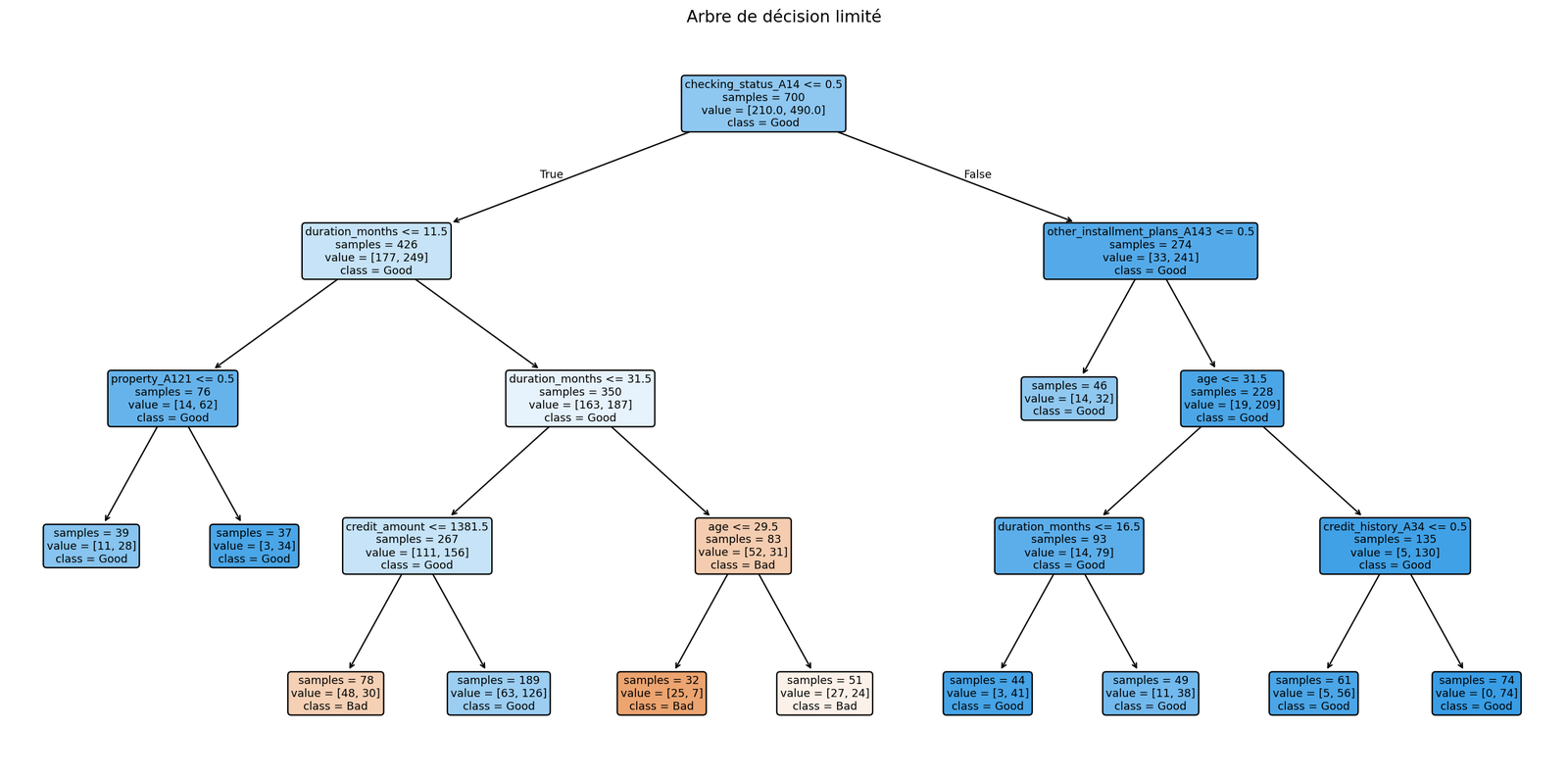
Pareto frontier scatter plot. Five models plotted with explainability score (X) and business score derived from cost (Y). Decision Tree in green at top-right; the other four models below or to the left, all dominated. — Pareto frontier: explainability score vs business score derived from the cost. Decision Tree alone in the non-dominated position.

The Decision Tree's explainability score is not subjective — the rules are the model. Every refusal is a path through the tree: checking_status_A14 ≤ 0.5 → duration_months > 11.5 → credit_amount > 1381.5 → age ≤ 29.5, and the outcome is read directly off the leaf. A risk officer can read it, defend it, and audit it without an external library. That is what the explainability score measures.

The trained decision tree for credit approval. Each node shows a feature condition, the number of samples reaching it, the class distribution, and the predicted class. Leaves are coloured by the majority class. — The trained decision tree. Every refusal is a chain of conditions readable end-to-end.

What's left for production

This is a one-week academic exercise; before it becomes a deployable system, three things need work. The cost matrix itself needs to be recalibrated against the bank's real P&L — the 5-to-1 asymmetry comes from the UCI dataset's documentation, not from production data. Three sensitive variables (personal_status_sex, age, foreign_worker) are kept in the model — refusal rates by sub-group need to be measured before any decision is automated. And the cost-sensitive threshold needs a drift policy: if the underlying default rate shifts, the optimal threshold shifts with it, and a pipeline that doesn't recalibrate silently turns into a calibration error.